As a teacher, you are constantly observing your class and seeing a variety of skill levels displayed by your students. Why not record those observations and use that data to help drive your instruction? Using a simple Google form can help keep all your formative or summative skill observation Physical Education assessments organized. This free tool takes the guesswork out of grading and gives you objective data you can use to give feedback to students and help guide your teaching. The great thing about using this form is that you can use this one, single form for EVERY skill assessment that you do for the entire year! No need to create a new form each time you assess. And, once you’ve made one, you can simply copy the form as a template for your next class, change the teacher name and student list and repeat this process until you have a form for every class you teach. Let me show you how…
Many of you have already created a free Google account. If you don’t have an account yet, you’ll need to create one first. CLICK HERE and follow the prompts to set one up. You’ll want to begin by opening your Google Drive and clicking on the +New button on the top left corner of your screen. Select “More” and then select “Google Forms”.
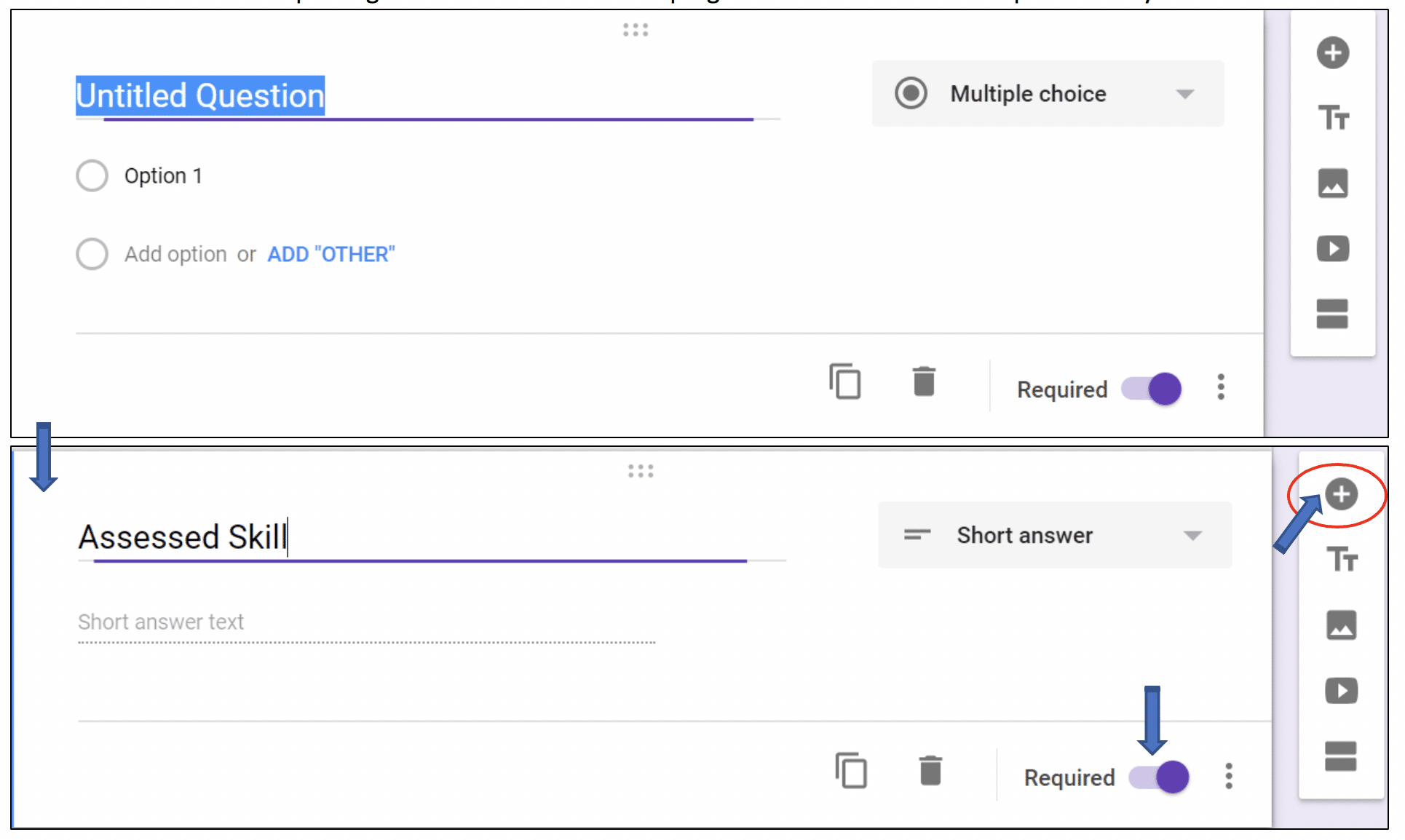
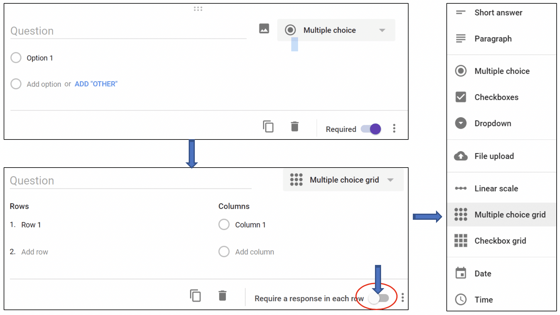
This second question is where we will add the student names and the grading scale you wish to use. We want to set this up using a “Multiple Choice Grid” format. Click on the question type (where it says “Multiple choice”) and select the “Multiple Choice Grid”. Switch the “Required” toggle to off. This way, if I don’t get a chance to assess the entire class during a given class period, I can still save/submit what I did and come back to the students I missed on another day.
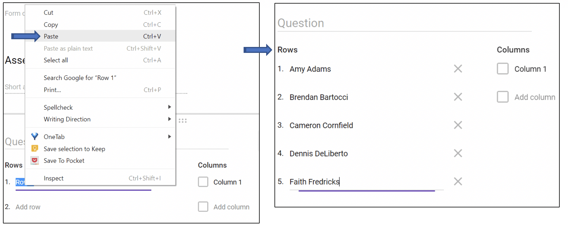
Now you are ready to add your students and your grading scale. Your students will be entered under the “Rows” and your grading scale will be entered under “Columns”. To streamline this step of the process, I find it best to have an electronic copy of your class roster available. I simply copy the student names from my spreadsheet and then click on “Row 1” and paste the names there. They will automatically populate with one name listed on each row! (time saver)
Next you add the grading scale you want to use to the “Columns” section. My District is set up with three grade descriptors, so I use a simple 3- point scale conversion to match the descriptors. I also add an “NA” for not assessed due to a student absence and a “MED” for any student that I can’t assess due to a medical reason.
The form is now complete and ready to start using! Click on the “eye” icon to preview your form.
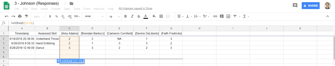
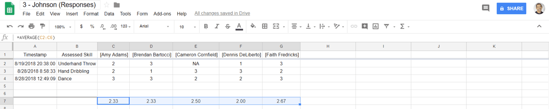
Then I copy and drag that “average” formula to all the other students across the row.

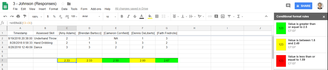
As an optional step, I color code the bottom “total average” row with a conditional formatting feature so that as scores are recorded, the cell will change color depending each student’s overall grade. I use green for my top grade (Demonstrates Consistency), yellow for my middle grade (Demonstrates Progress), and red for my low grade (Area for Improvement). On my 3-point scale, I break it down like this: 2.5-3 = Consistency, 1.6-2.49 = Progress, 1-1.59 = Improvement.
Here’s how I do that…first, select and highlight the entire row of averaged scores.
Next, click on FORMAT and select conditional formatting to get this option.
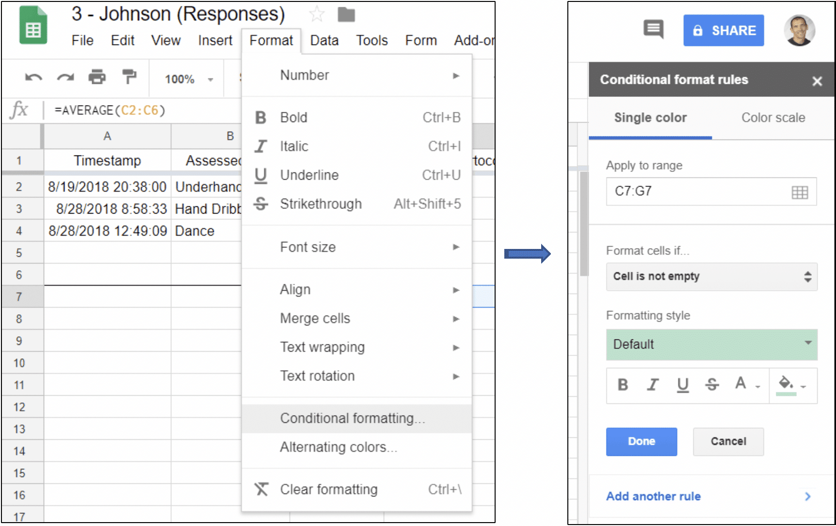
Next, set the “conditions” (or number ranges & colors) for your data. The first “rule” or condition will be to set your highest score. I select “Greater than or equal to” under the “Format cells if” selection box and type in 2.5. This means that all students who have an overall average of a 2.5 or higher will turn a certain color. I use the color green. Select the paint can and pick the color that works for you. When you’re finished setting the first color & number range, click “Add another rule”.
The second “condition/rule” you create is your middle score. Select “Is between” and enter the numbers 1.6 & 2.49. Select your color from the paint can (I use yellow) and then click “Add another rule”.
Finally, you will create or final “condition/rule” which will be your low score. Select “Less than or equal to” and enter the number 1.59. Select your color from the paint can (I use red) and the scores on your sheet are now formatted by color. The cells will now automatically change colors as more data is entered to reflect student performance.